Predicting Surge Pricing

There has been a boom in cab/ ride hailing business since a decade, so is the data. This Case Study was hosted as a Hackathon on Analytics Vidhya. This Business use case is on how to predict surge pricing in the taxi fare based on various metrics that cab aggregators capture.

Problem Statement

Sigma Cab Private Limited – a cab aggregator service. Their customers can download their app on smartphones and book a cab from any where in the cities they operate in. They, in turn search for cabs from various service providers and provide the best option to their client across available options. They have been in operation for little less than a year now. During this period, they have captured surge_pricing_type from the service providers.

In this project, we will build a predictive model, which could help them in predicting the surge_pricing_type pro-actively (multi-class classification). This would in turn help them in matching the right cabs with the right customers quickly and efficiently.

Prima facie

One can access the data from here by accepting t&c of AV: https://datahack.analyticsvidhya.com/contest/janatahack-mobility-analytics/

The initial understanding of Training and Test data reveals the following:

1. Train and Test data shows similar pattern in their mean and quartile distribution. This is great. We can assume that the test data is similar to that of Train and predictions on Train might work on Test
2. Train and Test have no empty records Train_ID, Train_Distance
3. We have few NaN in Type_of_Cab for both Train and Test. Lets create a new category ‘F’ with all the NaN values
4. Customer_Since_Months has few NaN values and replace them with 0. They are the first time users to this cab services.
5. Life_Style_Index, Confidence_Life_Style_Index. This is a proprietary value by the cab company and we have no idea how it is derived. Can think of omitting the NaN rows. Since, replacing them with 0 might mean something different. Or, can perform EDA and decide later. 
6. Destination_Type, Customer_Rating, Cancellation_Last_1Month have no missing values. 
7. Var1 is masked by the company and is very sparse. We definitely cant remove all records with NaN values and neither assume them to be 0. we could take a call on this after EDA. Perhaps remove this column.

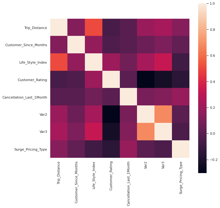
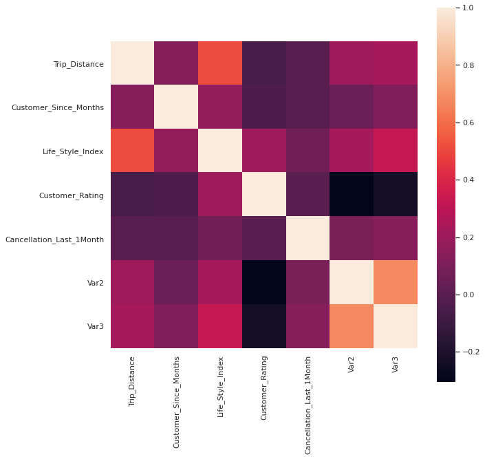
Correlation check

When checked the correlation of continuous variables in Train and Test data, its observed that Var2 and Var3 are correlated and the first can be removed.

Exploratory Data Analysis (EDA)

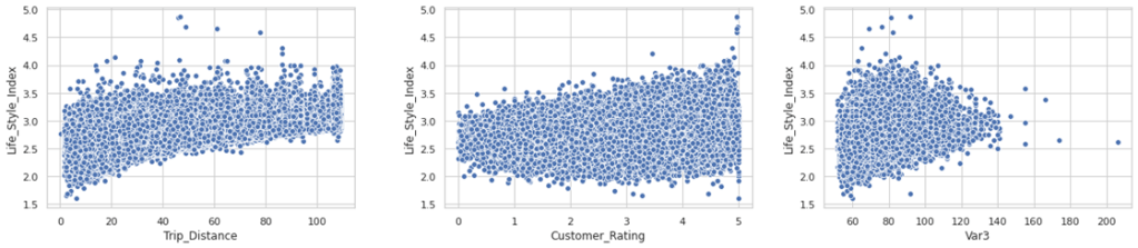
1. Life_Style_Index

From the 3 scatter plots, we can notice that most of the values of Life_style_index is distributed between 2 to 3.5

For simplicity, we fill assume NaN values with mode values for both Train and Test(2.7)

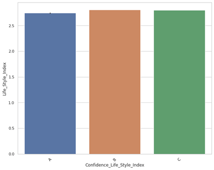
2. Confidence_Life_Style_Index

Look like the Confidence_Life_Style_Index is randomly assigned with equal distribution. For simplicity, lets equally assign A,B,C to the NaNs in the field.

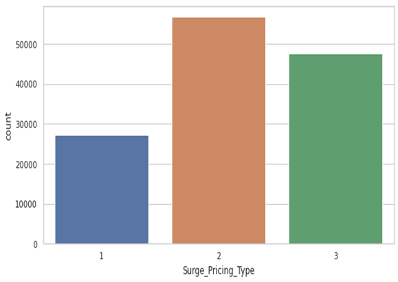
3. Surge_Pricing_Type

Not a large difference between the target values, and Sampling isn’t required. 

Modeling

1. Random Forest Classifier:

from sklearn.ensemble import RandomForestClassifier

rf_model = RandomForestClassifier()
rf_model.fit(X_train, y_train)

predictions_rf = rf_model.predict(X_test)

accuracy_score=metrics.accuracy_score(y_test, predictions_rf)

predictions = rf_model.predict(df_test)

df_submission.drop(columns='Surge_Pricing_Type', inplace=True)

df_submission['Surge_Pricing_Type']=predictions

df_submission.to_csv('/content/drive/My Drive/Projects/Hackathons/Analytics Vidya/Mobility/Data/Prediction_rf.csv')

Accuracy: 0.6857175407283637

2. XGBoost

from sklearn.multiclass import OneVsRestClassifier
from xgboost import XGBClassifier
from sklearn.preprocessing import MultiLabelBinarizer
from sklearn.model_selection import GridSearchCV

clf = xgb.XGBClassifier(objective='multi:softmax', n_estimators=27, 
                        num_classes=3)

clf.fit(X_train, y_train)  
pred=clf.predict(X_test)
pred

accuracy_score=metrics.accuracy_score(y_test, pred)
accuracy_score

Accuracy: 0.6835149812022937

3. XGBoost with GridSearchCV

xgb_model = xgb.XGBClassifier()
optimization_dict = {'max_depth': [2,4,6,None],
                     'n_estimators': [50,100,200,None]}

model = GridSearchCV(xgb_model, optimization_dict, 
                     scoring='accuracy', verbose=1)

model.fit(X_train, y_train)

print(model.best_score_)
print(model.best_params_)

pred=model.predict(X_test)
accuracy_score=metrics.accuracy_score(y_test, pred)

predictions_xgb = model.predict(df_test)

df_submission['Surge_Pricing_Type']=predictions_xgb

df_submission.to_csv('/content/drive/My Drive/Projects/Hackathons/Analytics Vidya/Mobility/Data/Prediction_xgb.csv')

Accuracy : 0.6966164128659856

Its to be noted that all these accuracy are for the Training data. The XGBoost with GridSearchCV gave a accuracy of 0.7015 on the Test data.

Conclusion

Perhaps the most important aspect of this exercise is the EDA. Having to understand which parameters/records can be omitted helps one quickly move to a better accuracy. This contest was slightly different as it involved mutliclass classification. There is a lot of scope in further understanding this project in terms of improving accuracy, feature importance and business implications/recommendations. Since it was time bound challenge, I haven’t explored those areas. However, I had tried a few other algorithms that can be observed in my github repository.

The contest challenge was to attain highest accuracy within a clocked time. This attempt gave me a rank of 113 of 8.5k participants.

Please feel free to provide your comments/ suggestions.