Minimizing Loan Evasions for a Bank – 1

Building Machine Learning Prediction model that minimizes the risk of Loan Evasions

Part – I

Have you ever applied for a loan? Do you remember what all information do Banks extract from individuals? Ever wondered how Banks utilize these information?

One of the leading Bank that I have worked with gets millions of applicants looking for loans of all kinds. Funding education, opening a small business, buying a car, planing a travel, gifting to someone, and so on. The Bank wasn’t sure how to decide on levying restrictions, which one would be a profitable lend and which one would default! The Bank wanted a system where they could screen an applicant based on the information that they provide and make decisions based on it.

After a couple of discussions with the Bank, I was provided with a ledger that had past loan applicants data with the defaulters information. A total of 0.33 Million applications with more than 150 different fields of information.

Based on the data provided, I had two ways to come up with such predictions. The Part-I focuses on utilizing categorical and continues variables as predictors and Part-II is about ‘text’ inputs as predictors.

You can access it here : Default Prediction – Part II

Dataset:
Here is a link to the Dataset: https://drive.google.com/file/d/1yucoB6Oo69js7vcaibDe_FVyo2-WkrWH/view?usp=sharing
(please email if you can’t download the file)

Before we move any further, here is the link to the Python Code.

Please note that this project is more about understanding the approach than just to code. I have skipped mentioning few of the ML models in this post, which can be accessed in my GitHub Repo.

Let me list out Table of Contents for a quick overview on what we are going to perform through this exercise.

Table of contents:

1. Data Pre-processing
2. Exploratory Data Analysis
3. Modeling with different Algorithms
   1. Logistics Regression
   2. Decision Tree
   3. Random Forest
   4. Support Vector Machines
   5. Single Layered NN
   6. Multi-Layered NN
   7. Gradient Boosting
   8. Bagging Classifier
   9. Bagging Classiefier with Decision Tree Classifier
   10. Voting Classifier
   11. AdaBoost Classifier
   12. Extra Tree Classifier
4. Analysis
5. Conclusion
   

1. Data Pre-Processing

As as first step, I’ve imported the data into a pandas dataframe. This can be done with the code given below.

data = pd.read_csv("/content/drive/My Drive/fullacc.csv")

Evaluating the kind of data types we have in the dataframe is a very important and initial steps to do. The following piece of code helps us to know the same. Here, we can see to have 150 total columns with both categorical and continues variables.

data.columns 

Index(['id', 'member_id', 'loan_amnt', 'funded_amnt', 'funded_amnt_inv',
       'term', 'int_rate', 'installment', 'grade', 'sub_grade',
       ...
       'orig_projected_additional_accrued_interest',
       'hardship_payoff_balance_amount', 'hardship_last_payment_amount',
       'debt_settlement_flag', 'debt_settlement_flag_date',
       'settlement_status', 'settlement_date', 'settlement_amount',
       'settlement_percentage', 'settlement_term'],
      dtype='object', length=150)

To be precise, we have 115 continues variables and 35 categorical variables. We can have a check on that by the following code.

data.describe() 

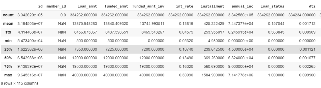
As a first step to feature extraction, lets check those predictor values (columns that are used to predict the default value) with data less than 90%. As a practice, we can consider those variables which have data availability greater than 80% (or) 85%. However, for this exercise, I’ve considered 90%. It was observed that 92 such columns didn’t had values more than 90%. Hence, dropping them. Hence, now we have 58 columns for the next process.

Based on the above filtering, following are the variables rejected:

1. ‘funded_amnt’, ‘funded_amnt_inv’ are directly related to loan_amnt, hence removing these.
2. ‘installment’ is rejected as I chose to keep term value.
3. ‘grade’, ‘sub_grade’, ’emp_title’, ‘url’,’title’, ‘zip_code’ are not considered for this analysis

This leaves 45 variables for our analysis. I’ve created a new dataframe ‘data_selected’ that carries all such variables.

data_selected = data[['id', 'loan_amnt', 'term',  'emp_length', 'home_ownership', 'annual_inc', 
                      'verification_status','issue_d' , 'loan_status', 'pymnt_plan', 'purpose', 
                       'addr_state', 'dti', 'delinq_2yrs', 'fico_range_low', 'fico_range_high', 'inq_last_6mths', 'open_acc', 'pub_rec', 'revol_bal', 
                      'revol_util', 'total_acc', 'initial_list_status', 'out_prncp', 'out_prncp_inv', 'total_pymnt', 
                      'total_pymnt_inv', 'total_rec_prncp', 'total_rec_int', 'total_rec_late_fee', 'recoveries', 
                      'collection_recovery_fee', 'last_pymnt_amnt', 'last_fico_range_high', 'last_fico_range_low', 'collections_12_mths_ex_med', 'policy_code', 
                      'application_type', 'acc_now_delinq', 'chargeoff_within_12_mths', 'delinq_amnt', 'pub_rec_bankruptcies', 
                      'tax_liens', 'hardship_flag', 'debt_settlement_flag']].copy()

Checking correlation between the variables is very important before we consider to do EDA. Correlation (positive or negative) establishes a linear relationship within the predictors. This check is a great way to impute variables and sometimes the presence of causal relationships.

Simple way of checking the correlation between variables is to draw a heatmap of variable correlation.

Following variables have shown relation with other variables and have been selected to drop from the data_selected dataframe. You might want to consider re checking the correlation after dropping these variables, just in case of any further correlation.

1. policy_code
2. fico_range_high
3. out_prncp_inv
4. ‘total_pymnt_inv’
5. ‘total_rec_prncp’
6. ‘total_rec_int’
7. ‘collection_recovery_fee’
8. ‘last_fico_range_low’
9. ‘total_pymnt’

There are other ways to check correlation. VIF(Variation inflation factor) is one such method which gives you a check on Multicolinearity. Here is a link to implementing it on python: https://etav.github.io/python/vif_factor_python.html

2. Exploratory Data Analysis(EDA)

In the pre-processing step, we could extract features that made more sense based on a few assumptions (like: data unavailability, correlation). In this step, we will further try reducing features that don’t make much sense and explore the parameters that we lock.

After giving a check on seeing missing records, I’ve found following variables in it: emp_length, annual_inc, dti, delinq_2yrs, inq_last_6mths ,open_acc,pub_rec.

As we can see that the missing records are in a few hundreds when compared to a 3 million records. Hence, omitting such records shouldn’t be a problem. However, make sure to ask the business/ domain expert on effects of amputating such records. For instance, we can see emp_length field has a few NaN values. However, according to Bank these are the individuals who are un-employeed. Hence removing such records wouldn’t make sense. Hence, such records should have NaN values replaced with 0.

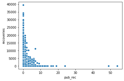
I wanted to understand relationship between continues variables with scatter plots.
The first graph shows the derogatory public records with respect to recoveries. As one can understand, accounts which had a bad records amounts to less recoveries. Hence, the company should continue giving loans to all those users who have shown less pub_rec values.
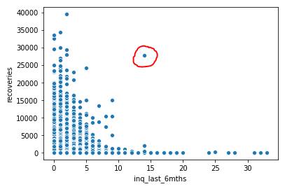
The second graph is between recoveries and inquiries made by Bank to the users(perhaps to recover). It is clear that most of the recoveries are made either initially or just after reminding them once / twice. However, we can also see that those users who have not paid have been called continuously. Hence, Bank should consider blacklisting such users.

An interesting observation on the outlier encircled in red. This doesn’t seem to be following the pattern. This might be a user who hasn’t paid until a lot of calls have been made by the company. Else consider this to be some error by a recovery agent while feeding a CRM. For the benefit of working with outliers, lets consider this to be a outlier and get rid of this from the records.

A couple of more graphs to understand categorical variables.

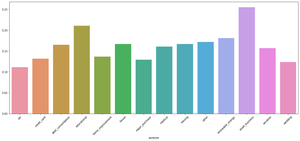
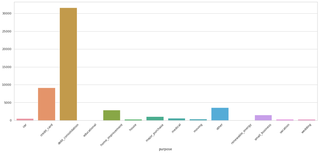
As you can infer from above chart, a lot of customers who default are from debt_consolidation category. However, a large percentage of detaults are from small business, followed by educational

Important to note that employee_length with null values are ‘unemployeed’ and should not be removed. Removing entries with no values for annual income, dti, delinq_2yrs, inq_last_6mths, open_acc, pub_rec (please note that the last 3 have no values to the same records).

I have conducted a few more EDA tasks that I am not including in this blog. Please feel free to check my github page.

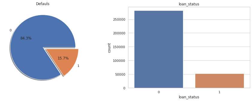
Lets also take a quick look at distribution of values (0’s and 1’s) to our target variable ‘loan_status’.

print(data_selected.groupby('loan_status').size()) #Checking counts of 0's and 1's in target variable

loan_status
0    281627
1     52462
dtype: int64

f,ax=plt.subplots(1,2,figsize=(16,5))
data_selected['loan_status'].value_counts().plot.pie(explode=[0,0.1],autopct='%1.1f%%',ax=ax[0],shadow=True)
ax[0].set_title('Defauls')
ax[0].set_ylabel('')
sns.countplot('loan_status',data=data_selected,ax=ax[1])
ax[1].set_title('loan_status')
plt.show()

Pictorial representation of imbalanced nature of target variable. We will have to employee sampling techniques to minimize this imbalance. We’ve chosen Up-Sampling technique.

Before sampling, lets also create a dummy variables for the categorical fields and avoid ‘dummy trap’ by dropping one dummy variable from each created.

#Creating dummy variables to all the categorical variables
data_selected = pd.get_dummies(data_selected, columns=['term', 'emp_length', 'home_ownership', 
'verification_status', 'pymnt_plan', 'purpose', 'initial_list_status', 
'application_type', 'hardship_flag', 'debt_settlement_flag'])

#Dropping one variable from each category to avoid dummy trap
data_selected.drop(['emp_length_7 years','verification_status_Verified', 'term_ 60 months', 'home_ownership_ANY' , 'pymnt_plan_y','purpose_car',
                    'initial_list_status_w', 'application_type_Joint App' , 'hardship_flag_Y', 'debt_settlement_flag_N'], axis=1, inplace = True)

Lets split the data into train and test. Considering only the train data, lets upsample it and join back to form new ‘selected_data’ dataframe.

#Up-Sampling the target variable
default_majority = train[train.loan_status==0]
default_minority=train[train.loan_status==1]
minority_upsampled = resample(default_minority,replace=True,n_samples=225262,random_state=44) 
minority_upsampled.shape[0]

train=pd.concat([default_majority,minority_upsampled])

Y_train = train.loan_status
Y_test = test.loan_status

X_train= train.drop('loan_status' , axis=1)
X_test = test.drop('loan_status', axis=1)

I have pickled the final train and test data for running it on different notebooks. Tip: If you are running different notebooks in parallel, consider pickling.

3. Modeling

I have considered different algorithms to learn how they behave with the given dataset. For all the models, the performance criteria selected are F1 Scores.

1. Logistics Regression:

One of the most simple and powerful algorithms for classification. I’ve created a model, fed the training and predicted the target variables. Now this model has given an accuracy of 0.934 to the test data, which is good. However, the F1 score of 0.812 doesn’t seem to be great.

logit = LogisticRegression()
logit.fit(X_train, Y_train)
Y_Pred=logit.predict(X_test)
logit.score(X_test, Y_test)


probs = logit.predict_proba(X_test)[::,1]

:
precision_score=metrics.precision_score(Y_test, Y_Pred)
recall_score=metrics.recall_score(Y_test, Y_Pred)
accuracy_score=metrics.accuracy_score(Y_test, Y_Pred)
f1_score=metrics.f1_score(Y_test, Y_Pred)

print("precision_score", precision_score,
      "\nrecall_score", recall_score,
      "\naccuracy_score", accuracy_score,
      "\nf1_score", f1_score,
      "\nAUC" , roc_auc_score(Y_test, probs))

Below is the confusion matrix, scores and ROC curve obtained:

array([[52938, 3427],
       [ 949, 9504]])

precision_score 0.9190335669494651 
recall_score 0.9534105041614848 
accuracy_score 0.9795713729833279 
f1_score 0.9359064656993944 
AUC 0.9808292680099435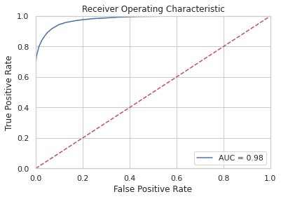

2. SVM (Support Vector Machine)

SVMs are memory and time consuming algorithms. Since we have around 3 million records, using SVM isn’t a great idea. However, just wanted to experiment. The following are the scores of the model

precision_score 0.9902805084041758 
recall_score 0.6366970517020367 
accuracy_score 0.8158027846551127 
f1_score 0.7750674570063175

3. Decision Tree:

from sklearn.tree import DecisionTreeClassifier
from sklearn.metrics import accuracy_score

#This piece of code is to check how accuracy varies by increasing tree depth. This will help us pick max_depth hyperparameter. 
max_depth = []
acc_gini = []
acc_entropy = []
for i in range(1,50):
 dtree = DecisionTreeClassifier(criterion='gini', max_depth=i)
 dtree.fit(X_train, Y_train)
 pred = dtree.predict(X_test)
 acc_gini.append(accuracy_score(Y_test, pred))
 ####
 dtree = DecisionTreeClassifier(criterion='entropy', max_depth=i)
 dtree.fit(X_train, Y_train)
 pred = dtree.predict(X_test)
 acc_entropy.append(accuracy_score(Y_test, pred))
 ####
 max_depth.append(i)
d = pd.DataFrame({'acc_gini':pd.Series(acc_gini), 
 'acc_entropy':pd.Series(acc_entropy),
 'max_depth':pd.Series(max_depth)})
# visualizing changes in parameters
plt.plot('max_depth','acc_gini', data=d, label='gini')
plt.plot('max_depth','acc_entropy', data=d, label='entropy')
plt.xlabel('max_depth')
plt.ylabel('accuracy')
plt.legend()

tree = DecisionTreeClassifier(max_depth= 7, max_features=20)

tree.fit(X_train, Y_train)

pd.Series(tree.feature_importances_, index=X_train.columns).sort_values(ascending = False)

predictions = tree.predict(X_test)
predictions[:5]
Y_test[:5]


confusion_matrix = confusion_matrix(Y_test, predictions)
confusion_df = pd.DataFrame(confusion_matrix, index=['Predicted Non-Defaulters','Predicted Defaulters'],\
                            columns=['Actual Non-Defaulters','Actual Defaulters'])

Following are the scores that I’ve got from DT:

precision_score 0.8332220924411814 
recall_score 0.9554194967951785 
accuracy_score 0.9631087431530426 
f1_score 0.8901466197245868 
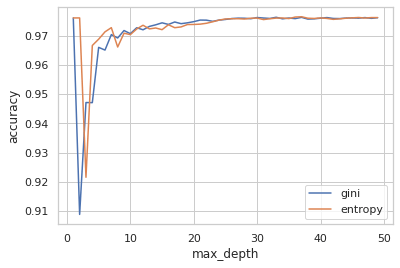
AUC 0.9599771128968352

Decision Trees have a lot of hyperparameters that one can tune. I’ve chosen max_depth and max_features for this analysis.

To find the max_depth, I’ve plotted it across accuracy. Below is the graph that shows the results. Ofcourse, for the most part of analysis, when max_depth is infinite, the accuracy of prediction is really good. However, it does get overfit and time consuming. However, we can see here at max_depth =7, the accuracy is really good.

In order to find the max_features, I had chosen GridSearch. I’ve got the best parameter value for max_features as 14. Hence, with these values, I re-ran the model to get the following scores:

precision_score 0.9273446545735238 
recall_score 0.9194489620204725 
accuracy_score 0.9761291867460864 
f1_score 0.9233799298650143

Further, to understand the importance/ effect of each predictor on target variable, we can use feature importance measure that gives values corresponding to it.

pd.Series(tree.feature_importances_, index=X_train.columns).sort_values(ascending = False)

recoveries                             0.827753
last_fico_range_high                   0.113253
last_pymnt_amnt                        0.039330
initial_list_status_f                  0.008738
debt_settlement_flag_Y                 0.005561
term_ 36 months                        0.001247
dti                                    0.001187
verification_status_Not Verified       0.001085
out_prncp                              0.000579
pymnt_plan_n                           0.000471
pub_rec                                0.000352
loan_amnt                              0.000162
purpose_major_purchase                 0.000110
total_acc                              0.000094
total_rec_late_fee                     0.000022
revol_bal                              0.000019
inq_last_6mths                         0.000019
home_ownership_OWN                     0.000009
annual_inc                             0.000007
emp_length_< 1 year                    0.000001

4. Random Forest:

Similar to that of a Decision Tree, I’ve selected max_depth as 14 and built the model.

from sklearn.ensemble import RandomForestClassifier
rf_model = RandomForestClassifier(max_depth=14)
rf_model.fit(X_train, Y_train)
predictions_rf = rf_model.predict(X_test)


precision_score=metrics.precision_score(Y_test, predictions_rf)
recall_score=metrics.recall_score(Y_test, predictions_rf)
accuracy_score=metrics.accuracy_score(Y_test, predictions_rf)
f1_score=metrics.f1_score(Y_test, predictions_rf)

print("precision_score", precision_score,
      "\nrecall_score", recall_score,
      "\naccuracy_score", accuracy_score,
      "\nf1_score", f1_score,
      "\nAUC" , roc_auc_score(Y_test, probs))

precision_score 0.9190335669494651 
recall_score 0.9534105041614848 
accuracy_score 0.9795713729833279 
f1_score 0.9359064656993944 
AUC 0.9808292680099435

4. Single Layer ANN:

This is a simple neural network that has one input and an output layer. We could also try adding early stop or dropouts. However, I haven’t applied them.

# Feature Scaling
from sklearn.preprocessing import StandardScaler
sc = StandardScaler()
X_train = sc.fit_transform(X_train)
X_test = sc.transform(X_test)

# Initialising the ANN
Defaulter_predictor = Sequential() 

# Adding the input layer and the hidden layer
Defaulter_predictor.add(Dense(input_dim=54, activation="relu", kernel_initializer="uniform", units=15))

# Adding the output layer
Defaulter_predictor.add(Dense(activation = 'sigmoid', kernel_initializer = "uniform", units = 1))

Defaulter_predictor.compile(optimizer = 'adam', loss = 'binary_crossentropy', metrics = ['accuracy'])

# Fitting the ANN to the Training set
Default= Defaulter_predictor.fit(X_train, Y_train, batch_size = 10, nb_epoch = 100)

Y_pred = Defaulter_predictor.predict(X_test)
Y_Pred = (Y_pred > 0.5)

precision_score=metrics.precision_score(Y_test, Y_Pred)
recall_score=metrics.recall_score(Y_test, Y_Pred)
accuracy_score=metrics.accuracy_score(Y_test, Y_Pred)
f1_score=metrics.f1_score(Y_test, Y_Pred)
print("precision_score", precision_score,
      "\nrecall_score", recall_score,
      "\naccuracy_score", accuracy_score,
      "\nf1_score", f1_score,
      "\nAUC" , roc_auc_score(Y_test, Y_Pred))

precision_score 0.953781056742975 
recall_score 0.841002582990529 
accuracy_score 0.9687509353766949 
f1_score 0.8938485002541943 
AUC 0.9167223506631879

4. Multi Layered ANN:

# Feature Scaling
from sklearn.preprocessing import StandardScaler
sc = StandardScaler()
X_train = sc.fit_transform(X_train)
X_test = sc.transform(X_test)

# Initialising the ANN
Defaulter_predictor = Sequential() 
# Adding the input layer and the hidden layer
Defaulter_predictor.add(Dense(input_dim=54, activation="relu", kernel_initializer="uniform", units=15))
# Adding the second hidden layer
Defaulter_predictor.add(Dense(activation = "relu", kernel_initializer = "uniform", units = 15))
# Adding the output layer
Defaulter_predictor.add(Dense(activation = 'sigmoid', kernel_initializer = "uniform", units = 1))

Defaulter_predictor.compile(optimizer = 'adam', loss = 'binary_crossentropy', metrics = ['accuracy'])
Defaulter_predictor.fit(X_train, Y_train, batch_size = 10, nb_epoch = 100)Y_pred = Defaulter_predictor.predict(X_test)
Y_Pred = (Y_pred > 0.5)

precision_score=metrics.precision_score(Y_test, Y_Pred)
recall_score=metrics.recall_score(Y_test, Y_Pred)
accuracy_score=metrics.accuracy_score(Y_test, Y_Pred)
f1_score=metrics.f1_score(Y_test, Y_Pred)
print("precision_score", precision_score,
      "\nrecall_score", recall_score,
      "\naccuracy_score", accuracy_score,
      "\nf1_score", f1_score,
      "\nAUC" , roc_auc_score(Y_test, Y_Pred))

precision_score 0.7560076775431862 
recall_score 0.9420262125705539 
accuracy_score 0.9433685533838188 
f1_score 0.8388278388278388 
AUC 0.94282185284786

In addition to these algorithms, I’ve also tried other Ensemble models like Gradient Boosting, Bagging Classifier, Bagging with Trees, Voting Classifier, AdaBoost, Extra Tree Classifier.

You can access the code here:

As we have listed in “2- Decision Tree Algorithm” (best score when compared with other algos) section, the Top 6 such parameters and why they are probably true:

1. recoveries: While connecting the dots backwards, one can understand that the amount recovered after charging off categorises if a user has paid/ defaulted.
2. last_fico_range_high: Certainly FICO are the most important parameter that indicates an individual’s credit health. Insurance/Creditors spend a lot on this area to well qualify the credit limit to an individual.
3. last_pymnt_amnt: Intuitively, someone who would be paying would show a sign of it by paying frequently. Hence, for sure this is an important predictor variable.
4. initial_list_status_f: Interesting to learn that Bank claims to have allocating fractional(f) and whole(w) randomly to their customers. However, a lot of claimed that its a scam! (https://forum.lendacademy.com/index.php?topic=4815.0). In general, whole accounts are considered to give great returns. Hence, this parameter might play an important role in defaulting (as this represent ‘fractional’)
5. debt_settlement_flag_Y: As a consequence of someone paying/ no-paying this value is flagged
6. term_ 36 months:For obvious reasons, it can be understood that term length helps one to repay back conveniently. Hence, this does surely make sense.

This important exercise helped us understand cleaning the data, looking for a right plot to tell the story encoded in data, understanding which predictors weigh less importance and getting rid of them, ofcourse modeling and hyperparameters tuning.